Epidemic modelingIntroduction
This year we have witnessed the rise of a global pandemic threat: a virus called SARS-CoV-2. In this lesson, we'll develop some of the basic elements of epidemic modeling, so that we can understand a small part of what public health researchers are looking at when they make projections and inform public policy.
It's worth mentioning from the outset that epidemic modeling is a deep and complex subject, and without substantial experience it's impossible to know when the results of a model are really reliable. Furthermore, even in the best case scenario, there can still be a lot of uncertainty. Nevertheless, an appreciation of some of the phenomena observed in the simplest epidemic models can help us better understand the considerations being weighed by decision makers.
How viruses spread
A single SARS-CoV-2 particle, called a virion, consists of genetic material in the form of
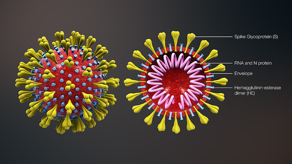
Figure 1.1. Image credit: scientificanimations.com (CC BY-SA)
When the virion enters a person's body, the spike proteins on its surface bind with receptors on the surface of a
Once the virus has reproduced sufficiently in a host, virus-laden droplets exit the host's body in various ways (coughing, sneezing, exhaling, etc.). These virus particles can
An infected person eventually recovers when their immune system develops
Exercise
List three ways in which the previous paragraph represents an oversimplification of what happens after a person is infected.
Solution. Here are some caveats:
- An infected person does not necessarily recover, since some people die with the illness.
- A person may become infected again if the virus mutates in such a way that the antibodies are no longer effective on the new
strain . - Antibodies don't last forever. A person may become infected again if they no longer have the antibodies they developed when they were originally infected.
Since the virus transmits discretely from one person to another, we can visualize the spread of the virus by drawing people as dots and transmission events as arrows connecting the dots. This mathematical structure is called a

Figure 1.2. The first person transmits to 3 people, then those people transmit to 1, 2, and 4 people, respectively, and so on. The average of these numbers (3, 1, 2, 4, etc.) is about 1.8.
Figure 1.2 suggests that when each infected person transmits the infection to 1.8 other people on average, the overall number of infected people

Figure 1.3. Starting from an infected population of size 40, each person transmits to about 0.5 people on average.
Figure 1.3 suggests that each infected person transmits the infection to 0.5 other people on average, the overall number of infected people
In summary, Figures 1.2 and 1.3 suggest the importance of the average number of people each infected person transmits to. If this number is large, then the infection tends to grow rapidly. If it's small, then the infection decreases rapidly.
Galton-Watson processes
Let's devise a simple probabilistic model for producing data along the lines of what's shown in Figures 1.2 and 1.3. We can use this model to experiment with the mean-transmission-number value.
Perhaps the simplest way to do this is to fix a
This random process is called a Galton-Watson process, and it has been studied since at least 1873. The results end up not depending very much on the exact details of the transmission distribution. Let's use with the
Exercise
Run the code cell below to see 16 runs of the Galton Watson process with initial population 1 and transmission mean 2.
Then adjust the values in the definition of the function sim to start with more infected people but a lower transmission mean.
(a) Which value of seems to mark the transition from growth to decay?
(b) If is on the larger side, the number of infectious persons
Note: the executable code cells are provided here for convenience, but if you'd prefer a notebook interface, you can launch a Jupyter notebook on Binder, with all packages pre-loaded, with one click).
Also, note that the cells may take some time to load initially, because a server is being launched for you in the background.
using Plots, Distributions
function galton_watson(n_generations; initial_population = 1, λ = 2)
    p = plot(legend = nothing, xaxis = nothing, yaxis = nothing)
    infectious_persons = 1:initial_population
    for generation in 1:n_generations
        infection_counts = [rand(Poisson(λ)) for person in infectious_persons]
        infection_totals = [0; cumsum(infection_counts)]
        for person in infectious_persons
            for new_person in 1:infection_counts[person]
                x = [generation - 1, generation]
                y = [person, infection_totals[person] + new_person]
                plot!(p, x, y, color = :MidnightBlue)
            end
        end
        infectious_persons = 1:sum(infection_counts)
    end
    p
end

sim() = galton_watson(5, initial_population = 1, λ = 2)
plot([sim() for _ in 1:16]..., layout = (4, 4), link = :both)
Solution.
(a) If , then more people are infected in each new time step (on average). Therefore, the infection typically spreads in this case. If , then the number of infected persons tends to decrease in each new generation. This comports with numerical experimention using the given code.
(b) Growth only usually occurs, since it can happen by luck that the virus is eradicted at a very early stage. Decay always occurs eventually in the scenario, since even if it happens to grow by luck initially, that luck does not persist forever.
It turns out that the intuition explored in the previous exercise is provably accurate (see the book Probability with Martingales by David Williams if you'd like to see a proof):
Theorem A Galton-Watson process eventually reaches extinction with probability 1 if and only if the mean of the transmission distribution is less than or equal to 1 (except in the trivial case where every person transmits to exactly 1 person with probability 1).
While the Galton-Watson model omits many important features of real-world epidemics, it illustrates one lesson which is valuable despite the oversimplification of the model: the fight is won or lost based on whether we can get each infectious person transmitting the infection to 1 or fewer other people on average.