The Data Science PipelineModeling
A machine learning model is a mathematical description of a relationship between random variables. In this section, we will focus on supervised learning, which is the task of predicting the values of one random variable given the values of others. We call the variable to predict the response variable and the other variables features.
We get information about the joint distribution of the features and response variable in the form of a tidy data frame whose rows represent independent samples from the distribution. These data are called training data.
Machine learning with no machine
Let's warm up with some supervised human learning.
Exercise
Fill in the missing data in the following data frame. Think of each row as having been randomly sampled from the distribution of a random vector in .
| x | y |
|---|---|
| 3 | 2 |
| 4 | 1 |
| -3 | 8 |
| 2 | 3 |
| 7 | -2 |
| 1 | |
| 6 |
In the data frame above, not much is clear about the distribution of the random variable . But it does seem reasonable to speculate that based on the available data. Based on this observation, we might choose to use as our prediction function for the problem of predicting based on the value of .
The situation where one random variable is strictly determined by another is rare in practice. Let's try a trickier version of the previous exercise:
Exercise
Fill in the missing data in the following data frame. Hint: it might help to make a scatter plot.
| x | y |
|---|---|
| 2 | 1 |
| 13 | 325 |
| 1 | 28 |
| 9 | 190 |
| 20 | 818 |
| 12 | 291 |
| 18 | 592 |
| 9 | 153 |
| -8 | 80 |
| 5 |
import plotly.express as px
from datagymnasia import show
import pandas as pd
df = pd.DataFrame({'x': [2, 13, 1, 9, 20, 12, 18, 9, -8],
                 'y': [1, 325, 28, 190, 818, 291, 592, 153, 80]})
show(px.scatter(df, x = 'x', y = 'y'))
The data in the table above were actually generated from a particular distribution, and the value of for the last observation happened to be 118. However, all you can really tell from the training data is that it looks like the value is probably between 0 and 200 or so. Because the
As illustrated in this example, when predicting one random variable given another random variable , we accept that we don't have enough information (even with perfect knowledge of the joint distribution of and ) to make an exact prediction. Instead, we typically estimate the
The human brain is remarkably well-suited to learning tasks like the one in the previous exercise. It's worth reflecting on some of its insights. Which of the following was closer to your mind's implicit model for how the random variables are related?


The advantage of the first model is that it's very
The advantage of the second model is that it passes through
The third model represents a compromise between underfitting and overfitting. It's curvy enough to match the training data reasonably well, but not so well that it will fail to generalize to new observations.
The tension between underfitting and overfitting is called the bias-complexity tradeoff, and it lies at the heart of machine learning.
Exercise
The following two figures represent two machine learning models for predicting a categorical variable. There are two features, represented by horizontal and vertical position in the plane. The response variable can be either 'red x' or 'blue o'. The prediction function is specified by color: points which fall in the red region are predicted to be red, and points which fall in the blue region are predicted to be blue.
Which model correctly classifies more training points?
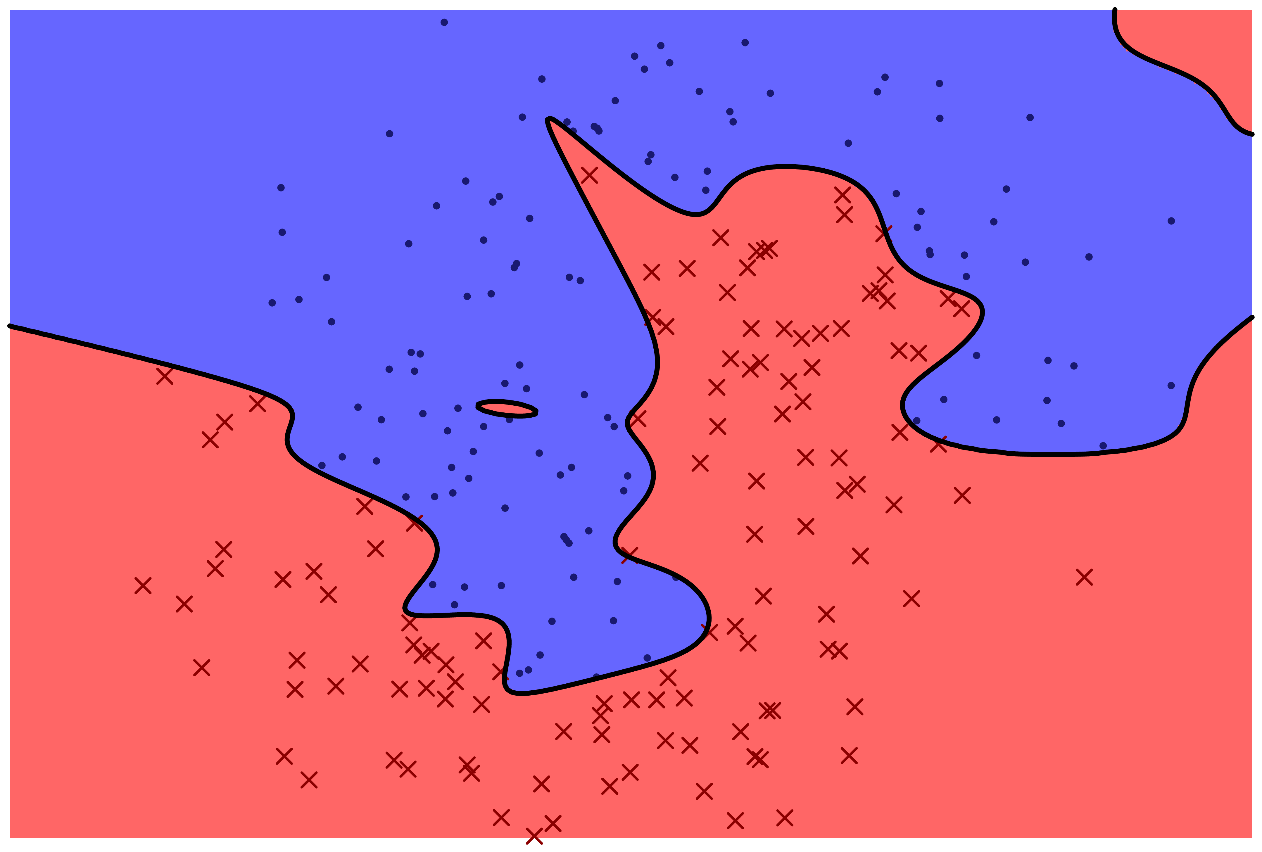
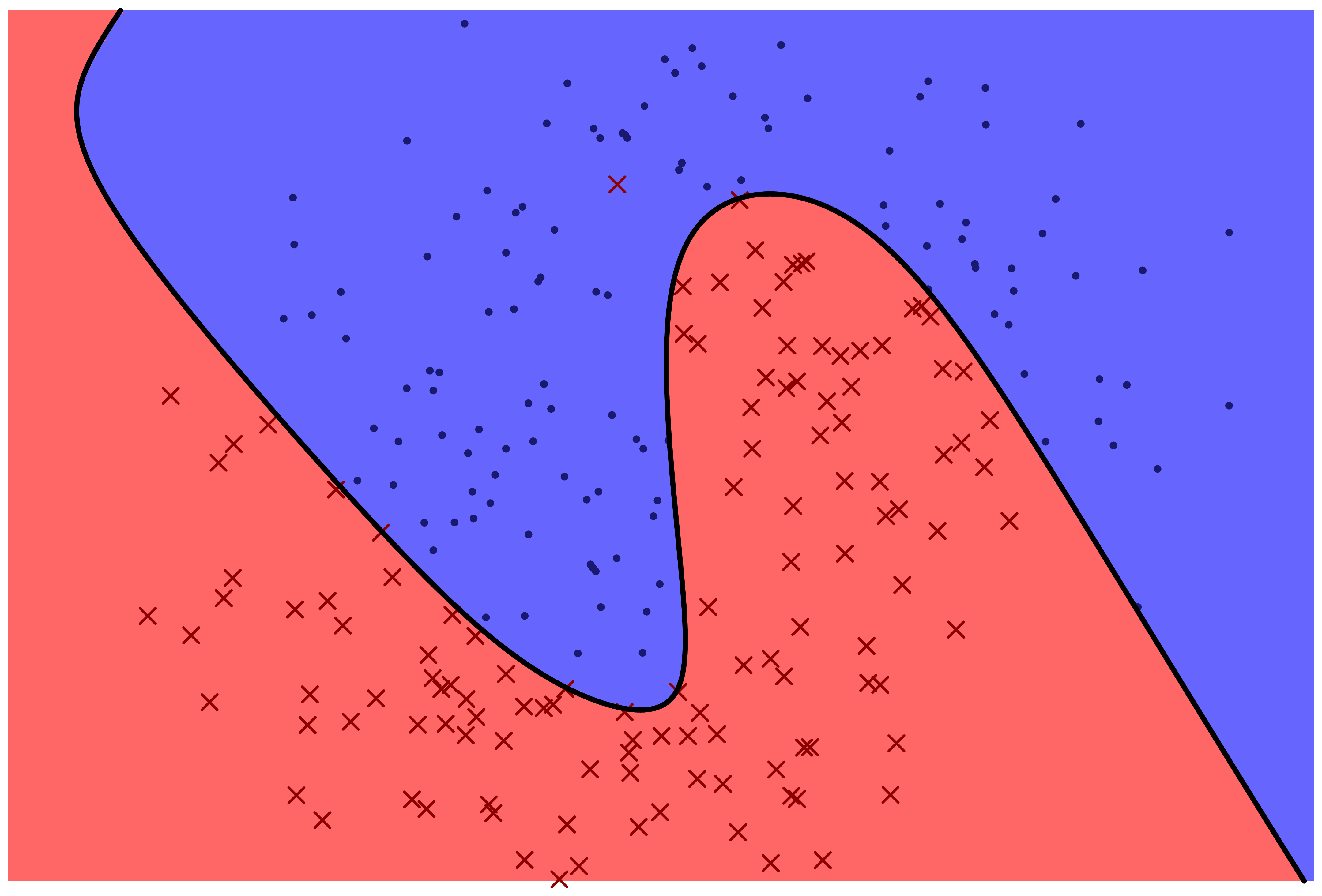
Which model is more likely to correctly classify a new observation based on its feature values?
Even with perfect information about the distribution that the data frame rows are sampled from, is it possible to correctly classify new observations with 100% accuracy?
If the response variable is categorical, then the prediction problem is called a
Scikit-Learn
The examples in the previous section hint at some of the disadvantages of the relying on the human brain to make data predictions: our ability to meaningfully visualize features maxes out pretty quickly. We can visualize only
So let's turn to doing machine learning with machines. Python's standard machine learning package is called Scikit-Learn. Let's see how it can be used to replicate the regression task you performed above, starting with linear regression.
Machine learning models in Scikit-Learn are represented as objects whose class reflects the type of estimator. For example, a linear regression model has class LinearRegression. Such objects can be fit to training data using the fit method, which takes two arguments: a two-dimensional array or data frame of features and a one-dimensional array of response values. Once the model has been fit, it can predict response values for a new two-dimensional array of features:
from sklearn.linear_model import LinearRegression
import pandas as pd
df = pd.DataFrame({'x': [2, 13, 1, 9, 20, 12, 18, 9, -8],
                  'y': [1, 325, 28, 190, 818, 291, 592, 153, 80]})
model = LinearRegression()
model.fit(df[['x']],df['y'])
model.predict([[5]])
This estimate ends up being significantly
Next let's use sklearn to fit the same data with a quadratic polynomial. There is no class for polynomial fitting, because polynomial regression is actually a special case of linear regression: we create new features by computing pairwise products of the original features and then fit a linear model using the new data frame. The coefficients for that model provide the quadratic coefficients of best fit for the original features.
In Scikit-Learn, creating new columns for the pairwise products of original columns is achieved using a class called PolynomialFeatures. To actually apply the transformation, we use the fit_transform method:
from sklearn.preprocessing import PolynomialFeatures
poly = PolynomialFeatures(degree=2)
extended_features = poly.fit_transform(df[['x']])
extended_features
Now we can use this new array to fit a linear model.
model = LinearRegression()
model.fit(extended_features,df['y'])
model.predict([[5]])
Oops! That didn't work because we need to process the input in the same way we processed the training data before fitting the model.
model.predict([[1,5,25]])
This model returns a value which is quite close to the conditional expectation of given , which is
Sklearn has a solution to the problem of having to apply the same preprocessing steps multiple times (once for training data and again at prediction time). The idea is to bind the preprocessing steps and the machine learning model into a single object. This object is called a pipeline. Let's do the same calculation again:
from sklearn.pipeline import Pipeline
model = Pipeline([('poly', PolynomialFeatures(degree=2)),
                  ('linear', LinearRegression(fit_intercept=False))])
model.fit(df[['x']],df['y'])
model.predict([[5]])
Much simpler! Note that we turned the LinearRegression model because the first step in the pipeline outputs a constant column (which plays the role of an intercept).
Having used toy data to go through some of the basics of sklearn, let's fit some models on a real data set on
Let's begin by looking at the dataset's documentation.
import pydataset
boston = pydataset.data('Boston')
pydataset.data('Boston',show_doc=True)Our goal will be to predict median housing prices (the column 'medv') based on the other columns in the data frame. However, we already have all of these values! If we want to be able to assess how well we are predicting median housing prices, we need to set some of the data aside for testing. It's important that we do this from the outset, because any work we do with the test data has the potential to influence our model in the direction of working better on the data we have than on actual fresh data. The arguments test_size and random_state specify the proportion of data set aside for testing (20%) and a seed for the random number generator to ensure we reproduce the same split if we run the code again.
from sklearn.model_selection import train_test_split
X_train, X_test, Y_train, Y_test = train_test_split(boston.drop('medv',axis=1),
                                                boston['medv'],
                                                test_size = 0.2,
                                                random_state = 42)
linear = LinearRegression()
linear.fit(X_train, Y_train)At this point we'd like to test our dflinear on the testing data we set aside. However, we should be very careful about doing that, because if we repeat that process on many models and select the best, then the testing data have effectively crept into the training loop, and we are no longer confident about how the model will perform on fresh data.
Instead what we'll do is carve out preliminary testing data from our training data. Then we'll follow the same fitting procedure to train a model on remaining training data. We can do this repeatedly to get a better sense for how our model tends to perform when it sees new data. This process is called cross-validation, and Scikit-Learn has built-in methods for it. We'll use a version called -fold cross-validation which partitions the training data into subsets called folds and trains the model with of the folds as training data and the last fold as test data. Each fold takes one turn as the test data, so you get fits in total.
We supply the model and the training data to the function cross_val_score. We use negative mean squared error for assessing how well the model fits the test data. The mean squared error refers to the average squared difference between predictions and actual response values, and this value is negated since Scikit-Learn's cross-validation is designed for the convention that a higher score is better (whereas un-negated squared error has the property that cv argument specifies the number of folds.
import numpy as np
from sklearn.model_selection import cross_val_score
scores = cross_val_score(linear, X_train, Y_train,
                         scoring="neg_mean_squared_error", cv=10)
linreg_cv_scores = np.sqrt(-scores)
linreg_cv_scores
The average value of the variable we're trying to predict is around
We can swap out the linear model for other sklearn models to see how they compare. For example, let's try decision tree regression, which can account for complex relationships between features by applying branching sequences of rules.
from sklearn.tree import DecisionTreeRegressor
decisiontree = DecisionTreeRegressor()
scores = cross_val_score(decisiontree, X_train, Y_train,
                         scoring="neg_mean_squared_error", cv=10)
tree_cv_scores = np.sqrt(-scores)
tree_cv_scores
import plotly.express as px
from datagymnasia import show
results = pd.DataFrame(
  {'scores': np.hstack((linreg_cv_scores,
                       tree_cv_scores)),
   'model': np.hstack((np.full(10,'linear'),
                       np.full(10,'tree')))}
)

show(px.histogram(results, x = 'scores', color = 'model', barmode = 'group'))Let's try one more model: the random forest. As the name suggests, random forests are made up of many decision trees.
from sklearn.ensemble import RandomForestRegressor
randomforest = RandomForestRegressor()
scores = cross_val_score(randomforest, X_train, Y_train,
                         scoring="neg_mean_squared_error", cv=10)
forest_cv_scores = np.sqrt(-scores)
forest_cv_scoresNow let's compare all three models:
results = pd.DataFrame(
    {'scores': np.hstack((linreg_cv_scores,
                          tree_cv_scores,
                          forest_cv_scores)),
     'model': np.hstack((np.full(10,'linear'),
              np.full(10,'tree'),
              np.full(10,'forest')))}
)
show(px.histogram(results, x = 'scores', color = 'model', barmode = 'group'))
According to this bar chart, the best model among these three is the
linear.fit(X_train, Y_train)
print(np.mean((linear.predict(X_test) - Y_test)**2))
decisiontree.fit(X_train, Y_train)
print(np.mean((decisiontree.predict(X_test) - Y_test)**2))
randomforest.fit(X_train, Y_train)
print(np.mean((randomforest.predict(X_test) - Y_test)**2))
Are these results expected? Discuss.
Hyperparameter tuning
A hyperparameter is a value which impacts the behavior of a model but which is held fixed during the fitting process. For example, if you fit a polynomial of degree to a set of data, then the coefficients of the polynomial are parameters and is a hyperparameter.
It's ultimately up to the data scientist to make good choices for hyperparameter values. However, you can automate this process by getting Scikit-Learn to search through a collection of values and return the best ones (selected according to cross-validation results).
The hyperparameters for a random forest include n_estimators (the number of trees in the forest) and max_features (the number of features that each branch in each decision tree is allowed to consider). GridSearchCV is a Scikit-Learn class for performing hyperparameter searches. It does cross-validation for every combination of the supplied parameters (hence grid in the name).
from sklearn.model_selection import GridSearchCV
param_grid = [
    {'n_estimators': [3, 10, 30], 'max_features': [2, 4, 6, 8]},
]
grid_search = GridSearchCV(randomforest, param_grid, cv=5,
                           scoring='neg_mean_squared_error')

grid_search.fit(X_train, Y_train)
grid_search.best_params_Although there's a lot more to know about data preparation and modeling, we've seen some of the basic elements in action: do any necessary preprocessing, prepare the data for modeling using a train-test split, fit a model to the data, assess models using cross-validation, and choose model hyperparameters using a grid search.
As you gain experience, the wrangling, visualization, and modeling phases will intertwine: you wrangle to get a better visualization and to prepare data for the model, you gain modeling insights from visualization, and your preliminary modeling results suggest visualizations to investigate. The process of navigating fluidly between wrangling, visualization, and modeling is called exploratory data analysis.