StatisticsEstimating Joint Densities
The following scenario will be our running example throughout this section. We will begin by assuming that we know the joint distribution of two random variables and , and then we will explore what happens when we drop that assumption.
Example
Suppose that is a random variable which represents the number of hours a student studies for an exam, and is a random variable which represents their performance on the exam. Suppose that the joint density of and is given by
Given that a student's number of hours of preparation is known to be , what is the best prediction for (as measured by mean squared error)?
Figure 1.1: The probability density function of the joint distribution of , where is the number of hours of studying and is the exam score.
Solution. The best guess of a random variable (as measured by mean squared error) is the expectation of the random variable. Likewise, the best guess of given is the conditional expectation of given . Inspecting the density function, we recognize that restricting it to a vertical line at position gives an expression which is proportional to the Gaussian density centered at . Therefore,
A graph of this function is shown in red in the figure below:
Figure 1.2: The conditional expectation of given , as a function of .
We call the regression function for the problem of predicting given the value of .
Given the distribution of , finding the regression function is a probability problem. However, in practice the probability measure is typically only known empirically, that is, by way of a collection of independent observations sampled from the measure. For example, to understand the relationship between exam scores and studying hours, we would record the values for many past exams (see Figure 1.3 below).
Figure 1.3: One thousand independent samples from the joint distribution of .
Exercise
Describe an example of a random experiment where the probability measure may be reasonably inferred without the need for experimentation or data collection. What is the difference between such an experiment and one for which an empirical approach is required?
Solution. There are many random experiments for which it is reasonable to use a measure derived from principle rather than from experimentation. For example, if we are drawing a card from a well-shuffled deck, or drawing a marble from a well-stirred urn, then we would assume that the probability measure is uniform. This assumption would lead to more accurate predictions than if we used an inferred measure based on repeated observations of the experiment. By extension, if we have many random variables whose distributions are known from principle and which are known from principle to be independent, then we know that their average is approximately normally distributed.
The key difference between these examples and those requiring an empirical approach is the use of symmetry. There is no a priori reason to believe that, for example, the possible scores on an exam are equally likely, or that an exam score is a sum of independent random variables.
You can convince yourself that , and indeed the whole joint distribution of and , is approximately recoverable from the samples shown in Figure 1.3: if we draw a curve roughly through the middle of the point cloud, it would be pretty close to the graph of . If we shade the region occupied by the point cloud, darker where there are more points and lighter where there are fewer, it will be pretty close to the heat map of the density function.
We will want to sharpen this intuition into a computable algorithm, but the picture gives us reason to be optimistic.
Exercise
In the context of Figure 1.3, why doesn't it work to approximate the conditional distribution of given using all of the samples which are along the vertical line at position ?
Solution. Because for almost all values of , there will be no points along the vertical line at position !
Kernel Density Estimation
The empirical distribution associated with a collection of observations from two random variables and is the probability measure which assigns mass to each location . The previous exercise illustrated shortcomings of using the empirical distribution directly for this problem: the mass is not appropriately spread out in the rectangle. It makes more sense to conclude from the presence of an observation at a point that the unknown distribution of has some mass near , not necessarily exactly at .
We can capture this idea mathematically by spreading out units of probability mass around each sample . We have to choose a function—called the kernel—to specify how the mass is spread out.
There are many kernel functions in common use; we will base our kernel on the tricube function, which is defined by
We define ; The parameter can be tuned to adjust how tightly the measure is concentrated at the center. Experiment with the slider below to get a feel for how changing affects the shape of the graph of .
We define the kernel function as a product of two copies of , one for each coordinate (see Figure 1.4 for a graph):

Figure 1.4: The graph of the kernel with XEQUATIONX2239XEQUATIONX.
Exercise
Is the probability mass more or less tightly concentrated around the origin when is small?
Solution. Note that as soon as either or is larger than . Therefore, all of the probability mass is less than units from the origin. So small corresponds to tight concentration of the mass near zero.
Now, let's place small piles of probability mass with the shape shown in Figure 1.4 at each sample point. The resulting approximation of the joint density is
Graphs of for various values of are shown below. We can see that the best match is going to be somewhere between the and extremes (which are too concentrated and too diffuse, respectively).
Figure 1.5: The density estimator for XEQUATIONX2241XEQUATIONX and . The last figure shows the actual density function.
Exercise
Estimate the best value of by eyeballing the figure above (the values of in the first four figures are 0.25, 1, 3, and 10. The last figure shows the actual density).
Solution. In the picture, it looks like the estimated measure is taking individual points too seriously, since there are lots of points with more mass around them than in the gaps between observations. In the picture, the mass looks way too spread out. Among the ones shown, appears to be the best.
We can take advantage of our knowledge of the density function to determine which value works best. In practice, we would not have access to this information, but let's postpone dealing with that issue till the next section.
We measure the difference between and by evaluating both functions at each point in a square grid and finding the sum of the squares of these differences. This sum is approximately proportional to
using LinearAlgebra, Statistics, Roots, Optim, Plots, Random
Random.seed!(1234)
n = 1000 # number of samples to draw

# the true regression function
r(x) = 2 + 1/50*x*(30-x)
# the true density function
σy = 3/2
f(x,y) = 3/4000 * 1/√(2π*σy^2) * x*(20-x)*exp(-1/(2σy^2)*(y-r(x))^2)

# x values and y values for a grid
xs = 0:1/2^3:20
ys = 0:1/2^3:10

# F(t) is the CDF of X
F(t) = -t^3/4000 + 3t^2/400

"Sample from the distribution of X (inverse CDF trick)"
function sampleX()
    U = rand()
    find_zero(t->F(t)-U,(0,20),Bisection())
end

"Sample from joint distribution of X and Y"
function sampleXY(r,σ)
    X = sampleX()
    Y = r(X) + σ*randn()
    (X,Y)
end

# Sample n observations
sample = [sampleXY(r,σy) for i=1:n]

D(u) = abs(u) < 1 ? 70/81*(1-abs(u)^3)^3 : 0 # tri-cube function
D(λ,u) = 1/λ*D(u/λ) # scaled tri-cube
K(λ,x,y) = D(λ,x) * D(λ,y) # kernel
kde(λ,x,y,observations) = sum(K(λ,x-Xi,y-Yi) for (Xi,Yi) in observations)/length(observations)
# `optimize` takes functions which accept vector arguments, so we treat
# λ as a one-entry vector
L(λ) = sum((f(x,y) - kde(λ,x,y,sample))^2 for x=xs,y=ys)*step(xs)*step(ys)

# minimize L using the BFGS method
λ_best = optimize(λ->L(first(λ)),[1.0],BFGS())
We find that the best value comes out to about . This is significantly smaller than our "eyeball" value of 3 from earlier, but not terribly far off.
Cross-validation
Since we only know the density function in this case because we're in the controlled environment of an exercise, we need to think about how we could have chosen the optimal value without that information.
One idea, which we will find is applicable in many statistical contexts, is to reserve one observation and form an estimator which only uses the other observations. We evaluate this density approximation at the reserved sample point, and we repeat all of these steps for each sample in the data set. If the resulting density value is consistently very small, then our density estimator is being consistently "surprised" by the location of the reserved sample. This suggests that our value is too large or too small. This idea is called cross-validation.
Exercise
Experiment with the sliders below to adjust the bandwidth and the omitted point
The density value at the omitted point is small when is too small because
We've decided we want the densities at the omitted points to be not too small, but we haven't specified an objective function to say exactly what we mean by that. It turns out that we can do this in a principled way, starting from the idea of integrated squared error.
Let's aim to minimize the loss (or error, or risk) of our estimator, which we define to be the integrated squared difference between and the true density . We can write this integral as
using
Recalling the expectation formula
we recognize the second term in the top equation as
We call
the cross-validation loss estimator. Let's find the value of which minimizes for the present example:
"Evaluate the summation Σᵢ f⁽⁻ⁱ⁾(Xᵢ,Yᵢ) in J(λ)'s second term"
function kdeCV(λ,i,observations)
    x,y = observations[i]
    newobservations = copy(observation)
    deleteat!(newobservations,i)
    kde(λ,x,y,newobservations)
end

# first line approximates ∫f̂², the second line approximates -(2/n)∫f̂f
J(λ) = sum([kde(λ,x,y,observations)^2 for x=xs,y=ys])*step(xs)*step(ys) -
        2/length(observations)*sum(kdeCV(λ,i,observations) for i=1:length(observations))
λ_best_cv = optimize(λ->J(first(λ)),[1.0],BFGS())
The cross-validated minimizing value is . Recall that the true minimizer is . So in this case, cross validation gets us quite close to the optimal value without needing to know the actual density. In fact, the cross-validation estimator performs well in general given enough data, in the following sense:
Theorem (Stone's Theorem)
Suppose that is a bounded probability density function. Let be the kernel density estimator with bandwidth obtained by cross-validation, and let be the kernel density estimator with optimal bandwidth . Then
converges in probability to 1 as . Furthermore, there are constants and such that and for large .
Nonparametric Regression
With an estimate of the joint density of and in hand, we can turn to the problem of estimating the regression function . If we restrict the density estimate to the vertical line at position , we find that the conditional density is
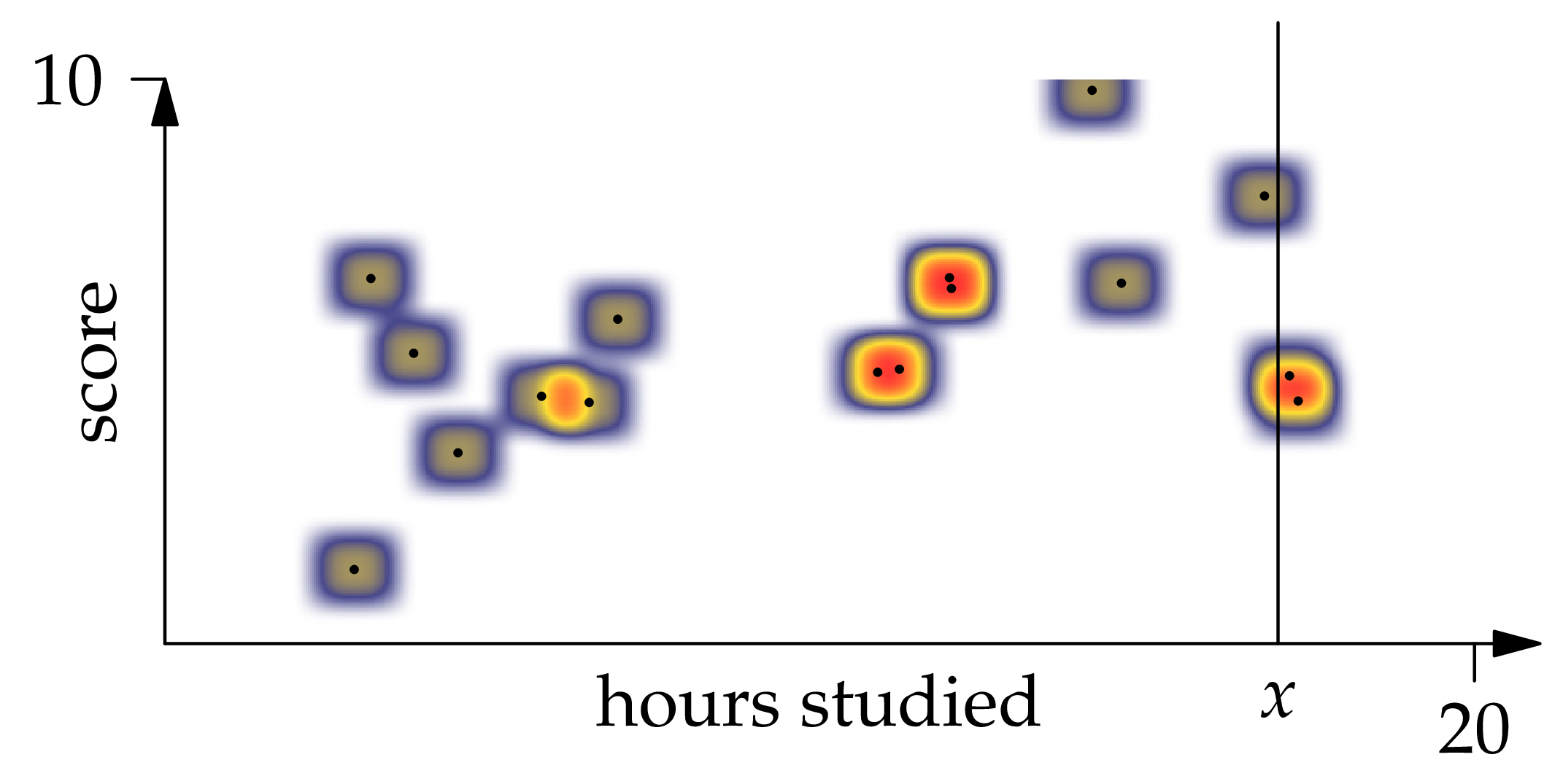
Figure 1.6: A kernel density estimator with 16 observations and XEQUATIONX2242XEQUATIONX.
So the conditional expectation of given is
Let's try to simplify this expression. Looking at Figure 1.6, we can see by the symmetry of the function that each observation contributes to the numerator of the above equation. To arrive at the same conclusion by manipulating the formula directly, we write
Then is the average of the probability measure with density centered at . Since is symmetric, this average is the center point .
Applying a similar idea to the denominator (note that instead of , we get the total mass 1 from integrating ), we find that
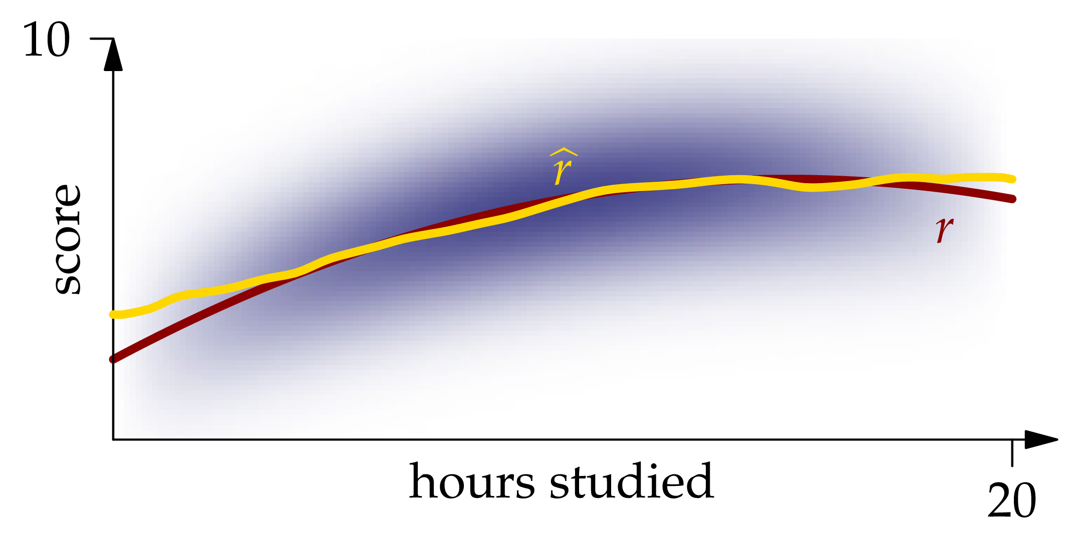
Figure 1.7: The Nadaraya-Watson estimator XEQUATIONX2240XEQUATIONX.
The graph of this function is shown in Figure 1.7. We see that it matches the graph of quite closely except near the ends of the interval.
λ = first(λ_best_cv.minimizer)
r̂(x) = sum(D(λ,x-Xi)*Yi for (Xi,Yi) in observations)/sum(D(λ,x-Xi) for (Xi,Yi) in observations)
scatter([x for (x,y) in observations],
        [y for (x,y) in observations],label="observations",
        markersize=2, legend = :bottomright)
plot!(0:0.2:20, r̂, label = L"\hat{r}", ylims = (0,10), linewidth = 3)
The approximate integrated squared error of this estimator is sum((r(x)-r̂(x))^2 for x in xs)*step(xs) = 1.90.
Kernel density estimation is just one approach to estimating a joint density, and the Nadaraya-Watson estimator is just one approach to estimating a regression function. In the machine learning course following this one, we will explore a wide variety of machine learning models which take quite different approaches, and each will have its own strengths and weaknesses.