Machine LearningA classification example: QDA
The task in the exam scores example is to predict a quantitative random variable given the value of a random variable Another common machine learning task is to predict a random variable taking values in a discrete set of labels. For example, we might want to identify users of a web app as academic, business, or personal users. Or we might want to classify medical devices as faulty or sound. These are called classification problems.
Exercise
Suppose that are random variables defined on the same probability space, and suppose that takes values in . For example, suppose that we select a forest animal at random and let be its weight and the kind of animal it is (where and correspond to and , respectively). Suppose that is a function which is intended to predict the value of based on the value of . Explain why the mean squared error is not a reasonable way to measure the accuracy of the prediction function.
Solution. The mean squared error penalizes a misclassification differently depending on how far apart the class labels are (for example, misclassifying a squirrel as a fox would be worse than misclassifying it as a bear).
As discussed in the first section, the most common way to judge a prediction function for a classification problem is the 0-1 loss, which applies a penalty of 1 for misclassification and 0 for correct classification:
Since it is typically not meaningful to put the possible classifications in order along an axis, we usually represent a data point's classification graphically using the point's shape or color. This allows us to use all of the spatial dimensions in the figure for the values, which is helpful if is multidimensional.
Example
Given a flower randomly selected from a field, let be its petal width in centimeters, its petal length in centimeters, and its color. Let
Suppose that the joint distribution of and is defined as follows: for any and color , we have
where and is the multivariate normal density with mean and covariance matrix . In other words, we can sample from the joint distribution of of and by sampling from {R, G, B} with probabilities 1/3, 1/6, and 1/2, respectively, and then generate by calculating , where is a vector of two standard normal random variables which are independent and independent of .
Three hundred observations from the distribution of are shown in the figure below.

Colors and petal dimensions of 300 randomly selected flowers.
Find the best predictor of given (using the 0-1 loss function), and find a way to estimate that predictor using the given observations.


We can visualize the joint distribution of flower dimension and color by representing as a color (as in the first figure) or using the third spatial dimension (as in the second figure).
Solution. As in the regression example, we can do a decent job of classification with our eyes. If is located where there are lots of green observations, we would predict its classification as green, and similarly for blue and red. Let's think about how to approach this task mathematically.
To start, let's proceed using our knowledge of the joint distribution of . The predictor which has minimal misclassification probability is the one which maps to the classification with maximal conditional probability given . For example, if the conditional distribution on given were , then we would guess a classification of
The conditional distribution of given is given by
for ; in other words, we compute the proportion of the probability density at the point which comes from each color .
Let's build a visualization for the optimal classifier for the flowers by coloring each point in the plane according to its classification. First, let's get 300 observations from the joint distribution of :
using Plots, StatsBase, Distributions, Random
Random.seed!(1234)
struct Flower
    X::Vector
    color::String
end
# density function for the normal distribution N
xgrid = 0:0.01:15
ygrid = 0:0.01:15
As = [[1.5 -1; 0 1],[1/2 1/4; 0 1/2], [2 0; 0 2]]
μs = [[9,5],[4,10],[7,9]]
Ns = [MvNormal(μ,A*A') for (μ,A) in zip(μs,As)]
p = ProbabilityWeights([1/3,1/6,1/2])
colors = ["red","green","blue"]
function randflower(μs,As)
    i = sample(p)
    Flower(As[i]*randn(2)+μs[i],colors[i])
end
flowers = [randflower(μs,As) for i in 1:300]
Next, let's make a classifier and color all of the points in a fine-mesh grid according to their predicted classifications.
predict(x,p,Ns) = argmax([p[i]*pdf(Ns[i],x) for i in 1:3])
function classificationplot(flowers,p,Ns)
    rgb = [:red,:green,:blue]
    P = heatmap(xgrid,ygrid,(x,y) -> predict([x,y],p,Ns),
          fillcolor = cgrad(rgb), opacity = 0.4,
          aspect_ratio = 1, legend = false)
    for c in ["red","green","blue"]
        scatter!(P,[(F.X[1],F.X[2]) for F in flowers if F.color==c], color=c)
    end
    P
end
correct(flowers,p,Ns) = count(colors[predict(F.X,p,Ns)] == F.color for F in flowers)
classificationplot(flowers, p, Ns)
We see that the optimal classifier does get most of the points right, but not all of them. correct(flowers,p,Ns) returns 265, so the optimal classification accuracy is 265/300 ≈ 88% for this example. Now suppose we don't have access to the joint distribution of , but we do have observations therefrom. We can estimate as the proportion of observed flowers of color . We could estimate the conditional densities using kernel density estimation, but in the interest of bringing in a new idea, let's fit a multivariate normal distribution to the observations of each color. Let's begin by approximating the mean of the distribution of red flowers, using the plug-in estimator:
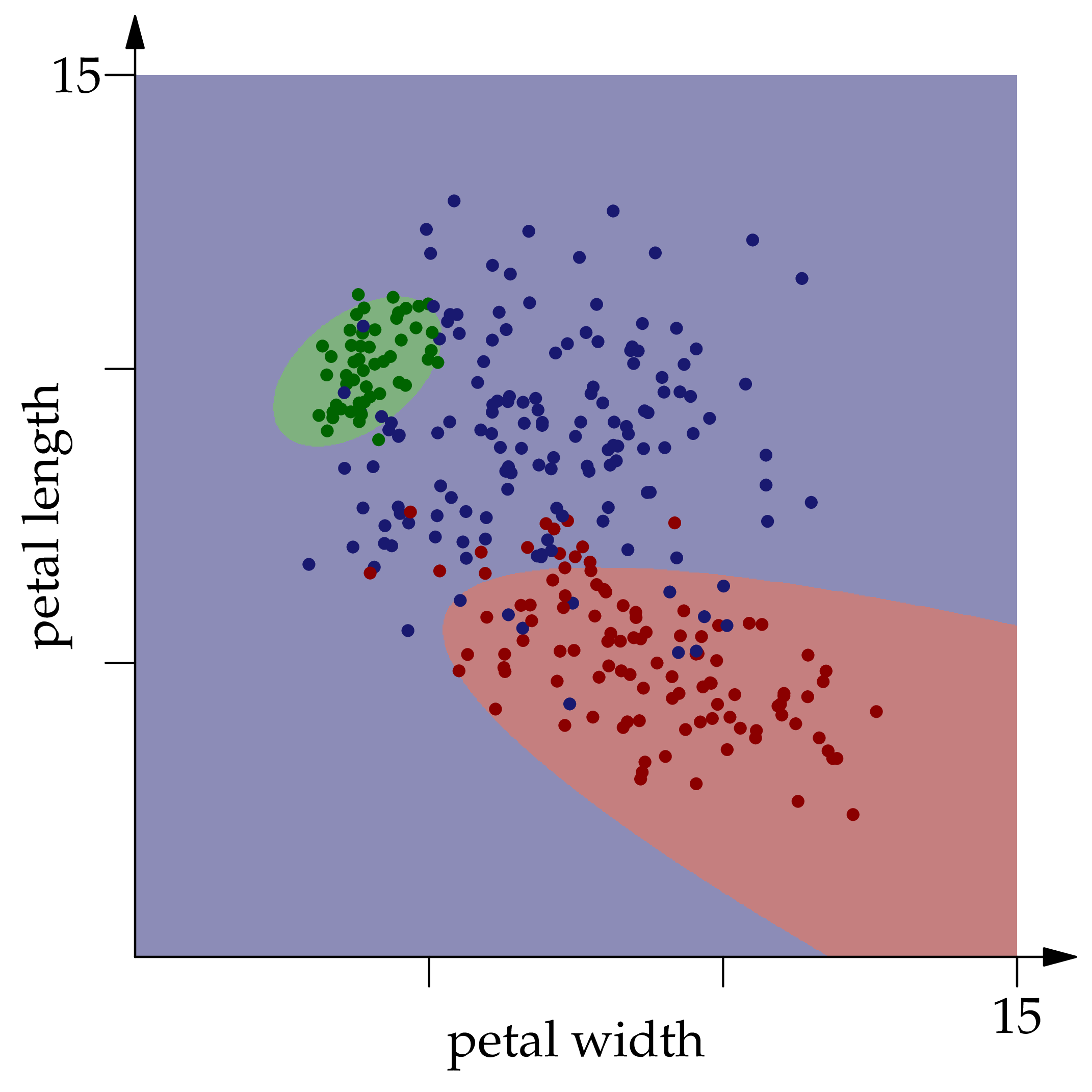
Each point in the square is colored according to the optimal classifier's prediction for the given $(x\_1,x\_2)$ pair.
and similarly for the other two colors. This formula estimates by using the empirical distribution as a proxy for the underlying distribution. Likewise, we approximate the red covariance matrix as
which evaluates the covariance matrix formula with respect to the empirical distribution.
     function mvn_estimate(flowers,color)
    flowers_subset = [F.X for F in flowers if F.color == color]
    μ̂ = mean(flowers_subset)
    Σ̂ = mean([(X - μ̂)*(X - μ̂)' for X in flowers_subset])
    MvNormal(μ̂,Σ̂)
end
colorcounts = countmap([F.color for F in flowers])
p̂ = [colorcounts[c]/length(flowers) for c in colors]
N̂s = [mvn_estimate(flowers,c) for c in colors]
classificationplot(flowers,p̂,N̂s)
The resulting plot looks very similar to the one we made for the optimal classifier, so this classifier does make the best prediction for most points .