Machine LearningDecision Trees
Your visual cortex has no difficulty using the following training data to predict the color of a point based on its and values:

A point falling in the second or fourth quadrants should be predicted to be
Exercise
Write a Julia function which accepts two arguments x1 and x2 and returns the predicted color. Assume that the vertical line separating the two colors in the first quadrant is .
function myprediction(x1,x2)
    # write code here
end

using Test
@test myprediction(-1,-2) == "green"
@test myprediction(0.5,-0.05) == "blue"
@test myprediction(0.45,0.25) == "red"
@test myprediction(0.65,0.8) == "green"
Solution. We can do this with a sequence of branching if statements:
function myprediction(x1,x2)
    if x1 < 0
        if x2 < 0
            "green"
        else
            "blue"
        end
    else
        if x2 < 0
            "blue"
        else
            if x1 < 0.5
                "red"
            else
                "green"
            end
        end
    end
end

using Test
@test myprediction(-1,-2) == "green"
@test myprediction(0.5,-0.05) == "blue"
@test myprediction(0.45,0.25) == "red"
@test myprediction(0.65,0.8) == "green"
The program you wrote in this exercise is an example of a decision tree. Decision tree classifiers map a feature vector to an output label using a flowchart of single-feature decisions.

A decision tree is a flowchart where each split is based on a single inequality involving a single feature.
Exercise
Which of the following are possible classification diagrams for a decision tree?


Solution. Only the first and third diagrams are possible. The second one would require making a decision based on the sum of the coordinates, which is not permitted (by the definition of a decision tree).
Training a Decision Tree
We were able to train a decision tree for the toy dataset above, but only by including a human in the training process. We'll need a more principled approach, for several reasons: (1) real-world data are almost always significantly messier than this example, (2) higher-dimensional feature vectors make visualization infeasible, and (3) we'll see that being able to train trees quickly gives us access to techniques which will tend to improve performance on real-world data sets.
The most commonly used decision-tree training algorithm, called CART, is greedy. At each node in the decision tree, we choose the next decision based on which feature and threshold do the best job of splitting the classes in the training data. To measure how well the classes have been divided, we define the Gini impurity of a list of labeled objects to be the probability that two independent random elements from the list have different labels: if are the proportions for the labels, then
For example, the Gini impurity of a list of 4 red objects, 2 green objects, and 3 blue objects is
The quantity that we minimize at each node in the decision tree is , where and are the proportion of training observations that go to the two child nodes and and are the child-node Gini impurities. Let's look at an example to convince ourselves that this is a reasonable quantity to minimize.
Exercise
Use the cell below to generate data in for which most of the points in the left half of the square are red and most of the points in the right half are blue. Consider splitting the set along a vertical line at position , and evaluate for that value of . Plot this function over the interval [0.05, 0.95].
using Plots
n = 500
X = [rand(n) rand(n)]
function pointcolor(x)
    if x[1] < 0.5
        rand() < 0.1 ? "blue" : "red"
    else
        rand() < 0.1 ? "red" : "blue"
    end
end
colors = [pointcolor(x) for x in eachrow(X)]
scatter(X[:,1], X[:,2], color = colors, ratio = 1,
size = (400,400), legend = false)We define p1, p2, G1 and G2 and plot the result:
using Statistics, LaTeXStrings
p1(x) = mean(row[1] < x for row in eachrow(X))
p2(x) = mean(row[1] ≥ x for row in eachrow(X))
function G(x, op) # op will be either < or ≥
    blue_proportion = mean(color == "blue" for (row,color) in zip(eachrow(X),colors) if op(row[1], x))
    red_proportion = 1 - blue_proportion
    1 - blue_proportion^2 - red_proportion^2
end
G1(x) = G(x, <)
G2(x) = G(x, ≥)
objective(x) = p1(x)*G1(x) + p2(x)*G2(x)
plot(0.05:0.01:0.95, objective, label = L"p_1G_1 + p_2G_2", legend = :top)
We see that it does have a minimum near the desired value of 0.5.
As long as the training feature vectors are distinct, we can always achieve 100% training accuracy by choosing a suitably deep tree. To limit the ability of the tree to overfit in this way, we supply a maximum tree depth. A maximum depth of 3, for example, means that no feature vector will be subjected to more than three decisions before being given a predicted classification.
Exercise
Use the code block below to train and visualize a decision tree on the iris dataset. How does the training accuracy vary as the maximum depth is adjusted?
using DecisionTree

features, labels = load_data("iris")

model = DecisionTreeClassifier(max_depth=3)
fit!(model, features, labels)
print_tree(model, 5)

sum(predict(model, features) .== labels)
Solution. We find that with a depth of 3, we can classify 146 out of 150 training observations correctly. Even with a depth of 1, we can get 100 out of 150 correct (since the setosas split perfectly from the other two species along the third feature).
Regression Trees
We can also solve regression problems with decision trees. Rather than outputting a classification at each terminal node of the tree, we output a numerical value. We will train regression trees greedily, as we did for classification trees: at each node, we look to identify the feature and threshold which does the best job of decreasing the mean squared error. Specifically, we minimize , where and are the proportions of observations which go to the two child nodes, and and are the variances of the sets of observations at each child node. We use mean squared error and variance interchangeably here, because the constant function which minimizes squared error for a given set of points is the
Exercise

Consider a set of data points in the unit square which fall close to the diagonal line . Among the functions on which are piecewise constant and have a single jump, which one (approximately) would you expect to minimize the sum of squared vertical distances to the data points? Confirm your intuition by running the code block below to plot MSE as a function of the jump location. (You can increase the value of to make the graph smoother.)
using Plots
n = 1_000
xs = rand(n)
ys = xs .+ 0.02randn(n)

function MSE(xs, ys, x)
    inds = xs .< x # identify points left of x
    p = mean(inds) # proportion of points left of x
    sum((ys[inds] .- mean(ys[inds])).^2) + # MSE
        sum((ys[.!inds] .- mean(ys[.!inds])).^2)
end

plot(0:0.01:1, x -> MSE(xs, ys, x))
Solution. We would expect the optimal threshold to be in the middle, at , so that one piece of the piecewise constant function can approximate half the points as well as possible, and the other piece can approximate the other half. Plotting the overall MSE as a function of the threshold x, we see that indeed the minimum happens right around .
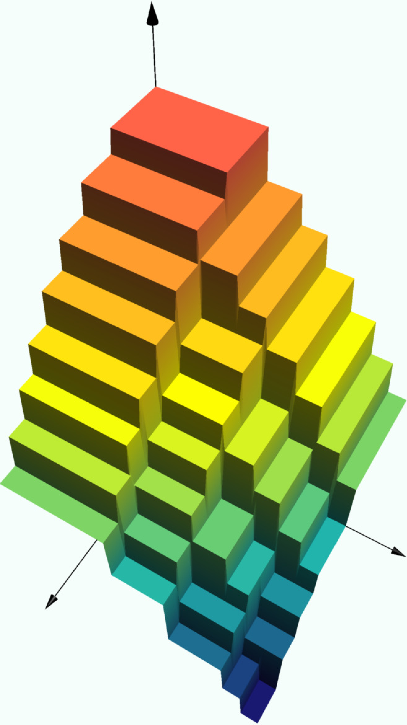
Exercise
Experiment with the depth in the code block below to see how the graph of the decision tree changes. The rectangles on which the prediction function is constant are always
using DecisionTree, Plots; pyplot()
n = 1000 # number of points
X = [rand(n) rand(n)] # features
y = [2 - x[1]^2 - (1-x[2])^2 + 0.1randn() for x in eachrow(X)] # response

model = DecisionTreeRegressor(max_depth=3)
fit!(model, X, y)
scatter(X[:,1], X[:,2], y, label = "")
surface!(0:0.01:1, 0:0.01:1,
         (x,y) -> predict(model, [x,y]))
heatmap(0:0.01:1, 0:0.01:1,
(x,y) -> predict(model, [x,y]),
aspect_ratio = 1, size = (500,500))