Machine LearningSupport Vector Machines
Logistic regression identifies linear decision boundaries by modeling the regression function . In this section, we will find decision boundaries directly based on desirable features of those boundaries. We begin with a warm-up exercise on the geometry of planes in .
Example
Find the distance from the plane to the point .
Solution. The vector is perpendicular to the given plane, so moving units directly away from some point in the plane means adding the vector
to that point. The value of the function is 6 for any point in the plane, and adding increases that value by :
Since the value of is equal to at the point , it changes by as you move from the nearest point on the plane to . We solve to find that the distance from the plane to the point is .
Example
Find the distance from the hyperplane to the point .
Solution. Generalizing the idea we developed in the previous problem, we can say that is the normal vector to the hyperplane, and moving units directly away from the hyperplane corresponds to adding to the value of . Therefore, we can check the value of the function at our point and divide by to find the distance from to the plane. So our distance formula is .
Example
Simulate data for a binary classification problem in the plane for which the two classes can be separated by a line. Write a Julia function for finding the thickest slab which separates the two classes.
Solution. Suppose that the observations are , where for each . Let us describe the separating slab as . The width of this slab is , by the preceding example. We can check whether a point is on the correct side of the slab by checking whether for points of class 1 and less than or equal to for points of class . More succinctly, we can check whether for all .
So, we are looking for the values of and which minimize subject to the conditions for all . This is a constrained optimization problem, since we are looking to maximize the value of a function over a domain defined by some constraining inequalities.
Constrained optimization is a ubiquitous problem in applied mathematics, and numerous solvers exist for them. Most of these solvers are written in low-level languages like C and have bindings for the most popular high-level languages (Julia, Python, R, etc.). No solver is uniformly better than the others, so solving a constrained optimization problem often entails trying different solvers to see which works best for your problem. Julia has a package which makes this process easier by providing a single interface for problem encoding (JuMP). Let's begin by sampling our points and looking at a scatter plot. We go ahead and load the Ipopt package, which provides the solver we'll use.
using Plots, JuMP, Ipopt, Random; Random.seed!(1234);
gr(aspect_ratio=1, size=(500,500))
Let's sample the points from each class from a multivariate normal distribution. We'll make the mean of the second distribution a parameter of the sampling function so we can change it in the next example.
function samplepoint(μ=[3,3])
    class = rand([-1,1])
    if class == -1
        X = randn(2)
    else
        X = μ + [1 -1/2; -1/2 1] * randn(2)
    end
    (X,class)
end
n = 100
observations = [samplepoint() for i in 1:n]
ys = [y for (x,y) in observations]
scatter([(x₁,x₂) for ((x₁,x₂),y) in observations], group=ys)
Next we describe our constrained optimization problem in JuMP. The data for the optimization is stored in a Model object, and the solver can be specified when the model is instantiated.
m = Model(with_optimizer(Ipopt.Optimizer,print_level=0))
We add variables to the model with the @variable macro, and we add constraints with the @constraint macro. We add the function we want to minimize or maximize with the objective macro.
@variable(m,β[1:2]) # adds β[1] and β[2] at the same time
@variable(m,α)
for (x,y) in observations
    @constraint(m,y*(β'*x + α) ≥ 1)
end
@objective(m,Min,β[1]^2+β[2]^2)
When we call solve on the model, it makes the optimizing values of the variables retrievable via JuMP.value.
optimize!(m)
β, α = JuMP.value.(β), JuMP.value(α)
Now we can plot our separating line.
l(x₁) = (-α - β[1]*x₁)/β[2]
xs = [-2,5]
plot!(xs,[l(x₁) for x₁ in xs], label="")
We can see that there are necessarily observations of each class which lie on the boundary of the separating slab. These observations are called support vectors. If a sample is not a support vector, then moving it slightly or removing it does not change the separating hyperplane we find.
The approach of finding the thickest separating slab is called the hard-margin SVM (support vector machine). A different approach (the soft-margin SVM) is required if the training observations for the two classes are not separable by a hyperplane.
Example
Consider a binary classification problem in for which the training observations are not separable by a line. Explain why
is a reasonable quantity to minimize.
Solution. Minimizing the first term is the same as minimizing the value of , which is the hard-margin objective function. The second term penalizes points which are not on the right side of the slab (in units of margin widths: points on the slab midline get a penalty of 1, on the wrong edge of the slab they get a penalty of 2, and so on). Thus this term imposes misclassification penalty. The parameter governs the tradeoff between the large-margin incentive of the first term and the correctness incentive of the second.
Example (Soft-margin SVM)
Simulate some overlapping data and minimize the soft-margin loss function. Select by leave-one-out cross-validation.
Solution. We begin by generating our observations. To create overlap, we make the mean of the second distribution closer to the origin.
observations = [samplepoint([1,1]) for i in 1:n]
ys = [y for (x,y) in observations]
scatter([(x₁,x₂) for ((x₁,x₂),y) in observations],group=ys)
Next we define our loss function, including a version that takes and together in a single vector called params.
L(λ,β,α,observations) =
    λ*norm(β)^2 + 1/n*sum(max(0,1-y*(β'*x + α)) for (x,y) in observations)
L(λ,params,observations) = L(λ,params[1:end-1],params[end],observations)
Since this optimization problem is unconstrained, we can use Optim to do the optimization. We define a function SVM which returns the values of and which minimize the empirical loss:
using Statistics, LinearAlgebra, Optim
function SVM(λ,observations)
    params = optimize(params->L(λ,params,observations), ones(3), BFGS()).minimizer
    params[1:end-1], params[end]
end
To choose , we write some functions to perform cross-validation:
function errorrate(β,α,observations)
    count(y * (β'*x + α) < 0 for (x,y) in observations)
end
function CV(λ,observations,i)
    β, α = SVM(λ,[observations[1:i-1];observations[i+1:end]])
    x, y = observations[i]
    y * (β'*x + α) < 0
end
function CV(λ,observations)
    mean(CV(λ,observations,i) for i in 1:length(observations))
end
Finally, we optimize over :
λ₁, λ₂ = 0.001, 0.25
λ = optimize(λ->CV(first(λ),observations),λ₁,λ₂).minimizer
β,α = SVM(λ,observations)
l(x₁) = (-α - β[1]x₁)/β[2]
xs = [-1.5,2]
plot!(xs, l, legend = false)
Kernelized support vector machines
Exercise

Support vector machines can be used to find nonlinear separating boundaries, because we can map the feature vectors into a higher-dimensional space and use a support vector machine find a separating hyperplane in that space.
Find a map from to a higher dimensional space such that the two classes shown in the figure can be separated with a hyperplane.
Solution. The distinguishing feature of the points is distance from the origin, so we supplement the features and with the combination . So our map is
We can see that the points can be separated by a plane in , so we could do a hard-margin SVM at this stage. To classify a test point , we can just check which side of the plane the point is on.
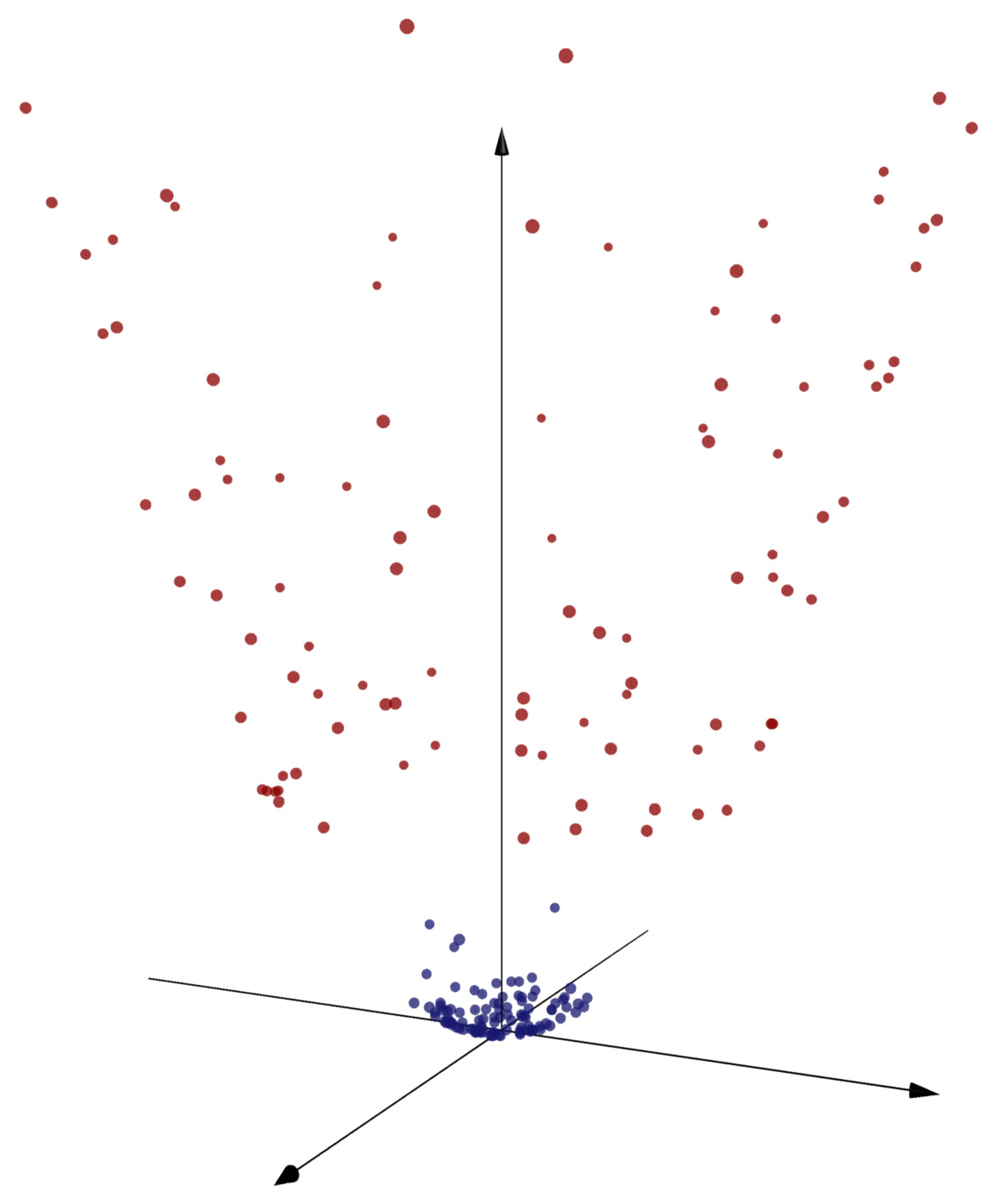
We can map points into a higher-dimensional space to achieve linear separation.
This example might have seemed a bit fortuitous, and it is structured so as to apparently rely on human insight to choose the appropriate map to . We can come up with a more general approach which leads to a new geometric perspective on kernelized support vector machines.
We begin with an overview of the mathematical theory underlying the support vector machine. This content tends to get notationally heavy, so we will adopt a vectorized notation which is more condensed and which also supports convenient translation to code.
We begin by slightly reformulating the soft-margin support vector machine. The SVM is a prediction function of the form
where and . To train a support vector machine on a set of training data , with and , we choose a value and solve the optimization problem
where indicates elementwise multiplication and indicates that the elementwise comparison holds for every element. The parameter governs the tradeoff between the margin width term and the classification penalty . Note that this is equivalent to minimizing
because if we multiply this expression by and set , and we can define to be the vector whose component is .
Next, we fold the constraints into the objective function by defining a function so that when and otherwise. Then our optimization problem is equivalent to
since the terms involving enforce the constraints by returning
Next, we swap the min and max operations. The resulting optimization problem—called the dual problem—is different, but the maximal value of the objective function in the new optimization problem does provide a lower bound for the first function. Here's the general idea (with as a real-valued function of two variables):
Furthermore, a result called
Performing the max/min swap and re-arranging terms a bit, we get
The first line depends only on , the second only on , and the third only on . So we can minimize the function over by minimizing each line individually. To minimize the first term, we rewrite as differentiate with respect to to get , which we can solve to find that .
The minimum of the second term is unless , because if any component of the vector multiplying were nonzero, then we could achieve arbitrarily large negative values for the objective function by choosing a suitably large value for in that component. Likewise, the minimum of the third term is unless is equal to
Therefore, the outside maximization over and will have to set and ensure that the equation is satisfied. All together, substituting into the objective function, we get the dual problem

Exercise
Show that we can give the dual problem the following interpretation, thinking of the entries of as weights for the training points:
- Each weight must be between 0 and
- Equal amounts of weight must be assigned in total to the +1 training points and to the -1 training points.
- The objective function includes one term for the total amount of weight assigned and one term which is equal to times the squared norm of the vector from the -weighted sum of negative training observations to the -weighted sum of positive training observations.
Note: the figure shows that values for each point, together with the -weighted sums for both classes (each divided by 3, so that their relation to the original points can be more readily visualized). The vector connecting these two points is .
Solution. The first statement says that , which is indeed one of the constraints. The second statement is equivalent to , since dotting with yields the difference between the entries corresponding to positive training examples and the entries corresponding to negative training examples.
The objective function includes one term for the total amount of weight (that's ), and one term which is , where . We can see that the vector is in fact the difference between the -weighted sums of the negative and positive training examples by writing as , where the +1 and -1 subscripts mean "discard rows corresponding to negative observations" and "discard rows corresponding to positive observations", respectively.
If we solve this problem, we can substitute to find the optimizing value of in the original problem. Although got lost in the translation from the original problem to the dual problem, we can recover its value as well. We'll do this by identifying points on the edge of the separating slab, using the following observation: consider a set of values which solves the optimization problem in the form
If is an index such that (in other words, the training point is inside the slab or on the wrong side of it), then must be zero, since otherwise we could lower the value of the objective function by nudging down slightly. This implies that .
Likewise, if component of is negative (in other words, the training point is safely on the correct side of the slab, and not on the edge), then we must have .
Putting these two observations together, we conclude that points on the edge of the slab may be detected by looking for the components of which are strictly between and . Since for training points on the edge of the slab, we can identify the value of by solving this equation for any index such that . We multiply both sides of the equation by to get , and that implies that .
In summary, the optimizing value of in the original problem may also be obtained looking at any component of
for which the corresponding entry of is strictly between 0 and . A couple caveats when working with solutions obtained numerically: we should (i) include a small tolerance when determining which entries of are deemed to be strictly between 0 and , and (ii) average all entries of for which is strictly between 0 and .
Exercise
Execute the code cell below to observe that the values of do indeed turn out to be 0 on the correct side of the slab, inside the slab or on the wrong side, and strictly between and only on the edge of the slab. Experiment with different values of .
include("data-gymnasia/svmplot.jl")
using Random; Random.seed!(1)

# number of training points of each class
n = 20
# generate training observations
X = [randn(n) .+ 1 randn(n) .+ 1
     randn(n) .- 1 randn(n)]
y = repeat([1,-1], inner = n)

# initialize and train an SVM:
S = SVM(X, y)
dualfit!(S, C = 0.5)

# visualize the SVM, together with annotations showing
# the η values
plot(S, (S,i) -> S.η[i])The Kernel Trick
The reason for formulating the dual problem is that it permits the application of a useful and extremely common technique called the kernel trick. The idea is that if we apply a transformation to each row of and call the resulting matrix , then the resulting change to the dual problem is just to replace with . This matrix's entries consist entirely of dot products of rows of with rows of , so we can solve the problem as long as we can calculate for all and in . The function is called the kernel associated with the transformation . Typically we ignore and use one of the following kernel functions:
where and are
To bring it all together, suppose that is a kernel function and is the resulting matrix of kernel values (where is the row of ). Then the support vector machine with kernel is obtained by letting be the optimizing vector in the optimization problem
The prediction vector for an feature matrix is
where is the matrix whose $(i,j)$th entry is obtained by applying to the row of and the row of , and where is any entry of
for which the corresponding entry in is strictly between 0 and .

Exercise
Consider applying an SVM with Gaussian kernel to a binary classification problem. Show that the function which maps a feature vector to its predicted class can be written as a composition of the signum function and a constant plus a linear combination of translations of the function . Where are these translations centered? Use this observation to reason about the behavior of the classifier when is large.
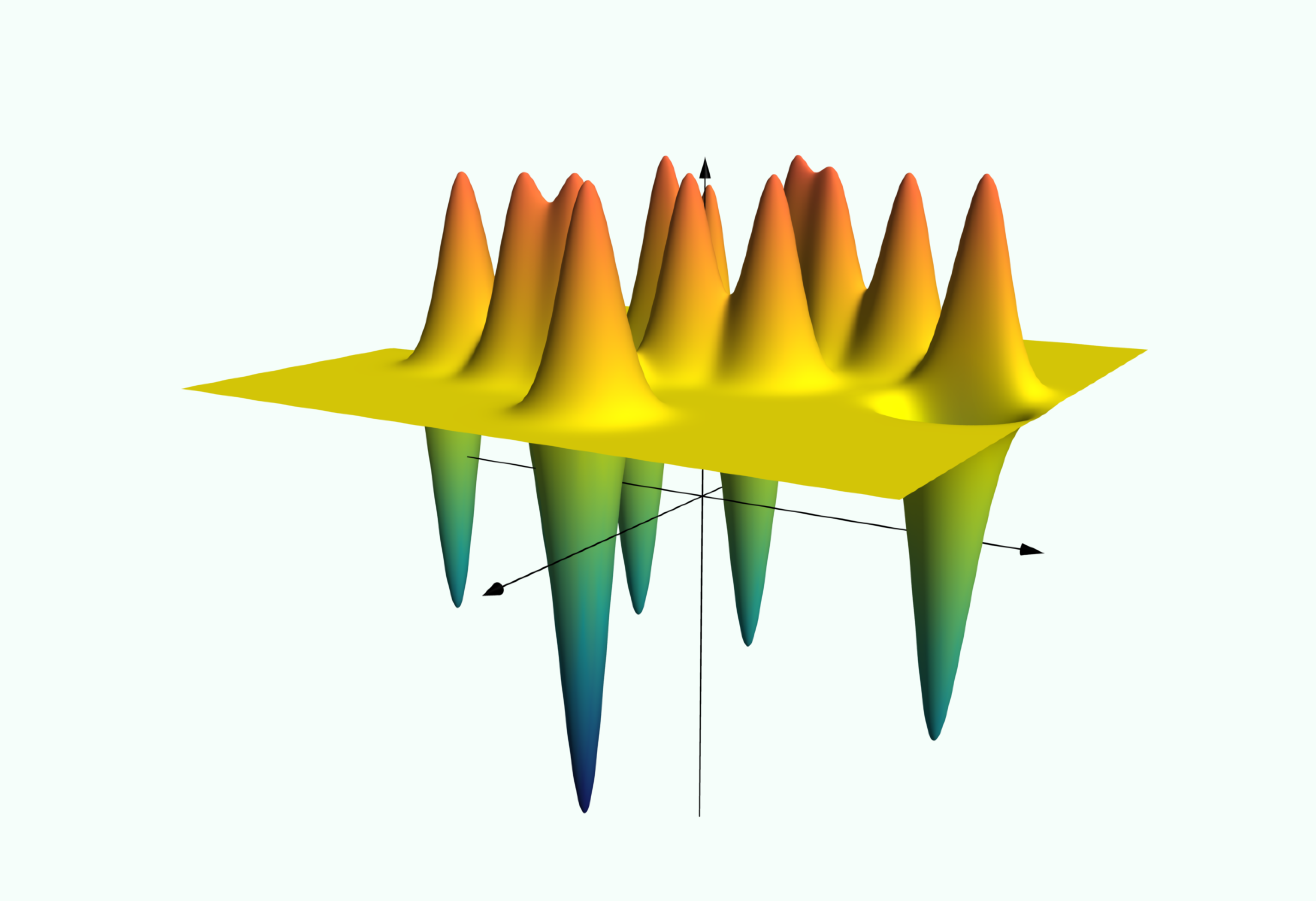
(In the scatter plot, the two axes represent features, and class is indicated with or . In the surface plot, the vertical axis represents predicted class (before the signum function is applied), while the other two axes represent features.)