Machine LearningDimension Reduction
Real-world data sets typically have many more than 2 or 3 features, which rules out direct use of the visualizations we've used for the examples we've seen so far. However, we can often apply a map from to a low-dimensional space which preserves much of the structure of the original data set.
Let's begin with an example where both the original space and the reduced space are low-dimensional.
Example
Finding a map from to such that each point shown can be reasonably accurately located if the value of is known. You may assume that the coordinates of the 100 points are stored in a matrix .

Solution. Consider the line which, roughly speaking, runs along the primary axis of the ellipse-shaped point cloud. If we know how far along this line one of the points is, then we know pretty accurately where it's located.
More precisely, for each point, we let be the orthogonal projection of onto the line . We would like to minimize the average squared error approximation .
We use an idea from singular value decomposition: the line through the origin which minimizes the sum of squared distances is the first column of in the singular value decomposition of . The only problem is that in this example this line does not pass through the origin. To deal with this issue, we recenter the points by finding the mean of the coordinates of the points and subtracting it from the coordinates of each point, so that the transformed points are centered at the origin. We then perform SVD on this new matrix to identify the line which minimizes the sum of squared distances to the points; now these lines all cross the origin. Once the best line's unit vector is known, we can determine for each point how far along the line its projection is by taking its dot product with . In other words, we can project all of the points onto by right-multiplying the matrix by .
The idea we developed in this example is called principal component analysis. We subtract off the means to center the point cloud, apply the singular value decomposition, and consider the first columns of the resulting matrix (these columns are called the principal components of the feature matrix). The desired dimension reduction map from to is represented by the matrix V[:,1:k]' (that is, the matrix obtained by removing all but the first columns of and then transposing).
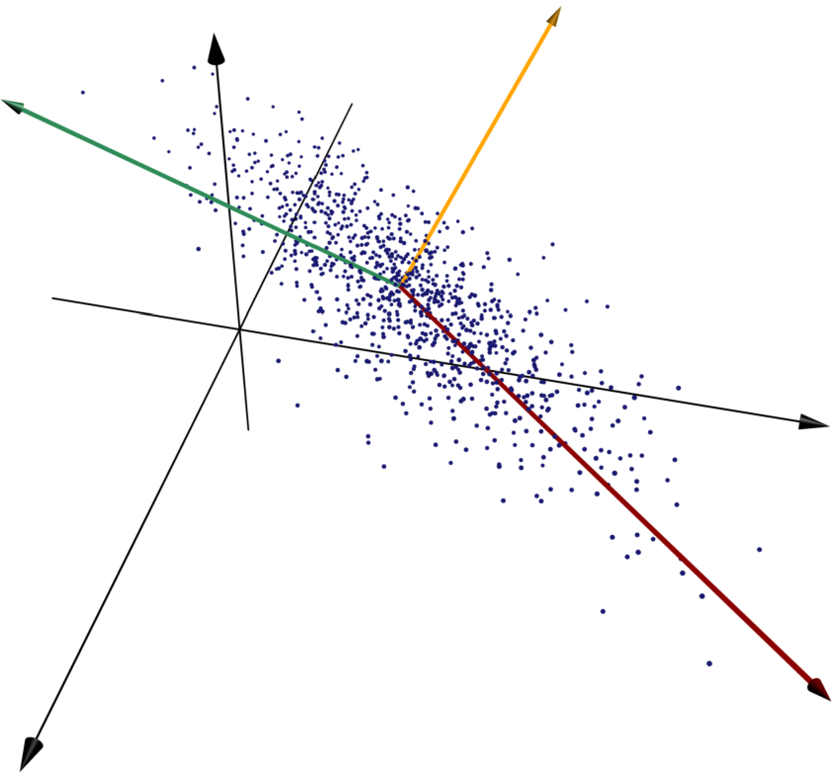
The three principal components of the given collection of points are shown in red, green, and gold, respectively. The red vector runs along the line whose sum of squared distances to the points is as small as possible, and the green vector minimizes the sum of squared distances to the points subject to the constraint of being orthogonal to the first vector.
Example
Apply principal component analysis to project the handwritten digit images in the MNIST dataset to the plane.
Solution. We begin by loading the dataset and reshaping the training data feature array.
using MLDatasets, Images, Plots
MNIST.download(i_accept_the_terms_of_use = true)
features, labels = MNIST.traindata(Float64)
A = reshape(features[:],28^2,60_000)'
Next, we define a custom function for displaying images. This function accepts a vector of length , it reshapes the entries into a square, and it returns an array of colors for display. If some of the components are negative, then negative and positive values are represented in different colors (red and blue, respectively). Otherwise, the image is displayed in grayscale.
function imshow(v)
    if any(v .< 0)
        (x -> x > 0 ? RGB(x,0,0) : RGB(0,0,-x)).(reshape(v./maximum(abs.(v)),(28,28))')
    else
        Gray.(reshape(v./maximum(abs.(v)),(28,28))')
    end
end
To perform principal component analysis, we take the column-wise mean with mean(A,dims=1) and subtract it from the matrix before performing the singular value decomposition.
using Statistics, LinearAlgebra
A = A[1:10_000,:] # make this computationally feasible on Binder
U, Σ, V = svd(A .- mean(A,dims=1))
imshow(V[:,1])
We can see the first principal component with imshow(V[:,1]), and similarly for the second principal component
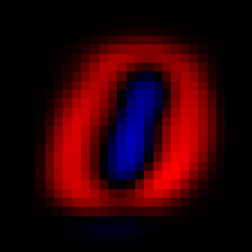
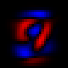
The first two principal components.
Finally, we project onto each of the first two principal components and make a scatter plot of the results. We set the marker size (ms) and the marker stroke width (msw) so we can see the colors of the points more clearly.
n = 5000
scatter(A[1:n,:]*V[:,1],
        A[1:n,:]*V[:,2],
        group=labels[1:n],
        markersize=2,
        markerstrokewidth=0)
We can see that some digits cluster apart from the other digits (like 1), while others remain heavily overlapping.
t-SNE
In this section we discuss a popular dimensionality reduction technique which is often more effective than principal component analysis at discovering structure in the dataset. The idea is to choose a map which attempts to preserve pairwise similarity of the data points. The version we present is called -SNE, which is short for -distributed stochastic neighbor embedding.
Suppose that is a set of points in . We begin by fixing a parameter of the model, called the perplexity . Given , we define
for , and for all . This quantity measures the similarity of distinct points and : if is closer to (compared to how close other points are to ), then is closer to 1. If is far from , then is close to 0.

Example
Consider the points , , , and . Find for each value of in .
Solution. We define a function to compute .
x = [[0,0],[0,1],[1,1],[4,0]]
f(x,y,σ) = exp(-norm(x-y)^2/(2σ^2))
P(x,i,j,σ) = f(x[i],x[j],σ) / sum(f(x[k],x[j],σ) for k in 1:length(x) if k ≠ j)
[P(x,2,1,σ) for σ in [0.25, 1, 2, 100]]
We find that , , , and .
We can see from this calculation that serves as the unit with respect to which proximity is being measured. If is very large, then all of the points are effectively close to , so the values of are approximately equal for . If is very small, then is close to 1 for 's nearest neighbor and is close to 0 for the other points.
For each from 1 to , we define to be the solution of the equation
The quantity on the left-hand side is called the Shannon entropy, and it measures how evenly distributed the values are. We fix the perplexity for each to ensure that the function avoids the extremes of too heavily concentrating its values on a small number of 's or spreading out its values too evenly across all of the 's.
We will denote by the images of the points under a map from the original feature space to a lower-dimensional Euclidean space (typically the plane or 3D space). We won't bother trying to define our dimension reduction map on the whole feature space; rather, we will let the domain of the map be just the set of training points. We begin by defining
These quantities measure the pairwise similarity of the points , analogously to . Notice, that rather than using a Gaussian function to measure neighborliness, we're using the Cauchy density . (As an aside, the Cauchy distribution is also known a the distribution with one degree of freedom, and that's where we get the in the name -SNE).
We measure how well the similarities match the similarities using the cost function
Finally, we use gradient descent to find values for the image points which minimize this cost function. Note that, since our dimension reduction map is only defined on the training points, we can think of the image coordinates as the parameters of the map and perform the gradient descent steps on the image coordinates. You can think of this visually as moving the locations of the points about freely so as to try to get the value of the cost function to go down. The following animation shows this process in action:
This animation comes from a blog post by Chris Olah, which contains many other animations and discussion of PCA, t-SNE, and related models.
Exercise
Why might it valuable to use the heavier tailed Cauchy function to compute the 's?
Solution. If two points which are supposed to be close are very far apart, the gradient of the Gaussian measuring their neighborliness will be tiny (since the Gaussian has derivative extremely close to zero outside of a small zone around the origin). This effect is much less pronounced with the Cauchy function, so the gradient signal in the optimization process is stronger.
Lastly, we note that the version of t-SNE proposed in the original t-SNE paper actually uses symmetrized versions of the 's and 's that they call and . (Symmetric means that and .) This version has some technical advantages and gives similar results to the asymmetric version discussed above.
Example
Use the Julia package TSne to plot a two-dimensional -SNE embedding of the first 2000 images in the MNIST data set.
Solution. We call the tsne function on the first rows of the MNIST matrix A defined above.
using TSne, Random
Random.seed!(123)
n = 2000
Y = tsne(A[1:n,:])
scatter(Y[:,1],Y[:,2],
        group=labels[1:n],
        ms=2,msw=0)
Congraulations! You've finished the Data Gymnasia Machine Learning course.